Abstract
Pattern formation in biological systems through chemoattractant-cell interactions represents a fundamental mechanism underlying numerous developmental and physiological processes. This paper presents a comprehensive study of partial differential equation (PDE) models describing pattern formation dynamics, focusing on three-PDE system in one spatial dimension. We employ the Method of Lines (MOL) for numerical solutions and compare results with two other numerical approaches and machine learning approach. Our analysis demonstrates the effectiveness of both traditional numerical methods and modern ML techniques in capturing complex spatiotemporal patterns. The study reveals critical parameter regimes for pattern formation and provides insights into the underlying biological mechanisms. Simulation results show good agreement between numerical and ML solutions, with computational efficiency gains observed in the machine learning approach.
Introduction
Pattern formation in biological systems is a ubiquitous phenomenon that underlies many critical processes, from embryonic development to wound healing and tumor growth. The interaction between cells and chemical signals, particularly chemoattractants and stimulants, plays a crucial role in organizing cellular behavior and generating complex spatiotemporal patterns.
Mathematical modeling of these phenomena typically involves systems of partial differential equations that capture the dynamics of cell density, chemical concentrations, and their mutual interactions. The complexity of these models arises from nonlinear coupling terms, diffusion processes, and reaction kinetics that operate across multiple spatial and temporal scales.
This study focuses on PDE models describing how cells interact with chemoattractants and stimulants in one-dimensional space. We investigate three-PDE system, starting from basic diffusion equations and progressively incorporating nonlinear terms that capture essential biological mechanisms such as chemotaxis, cell proliferation, and chemical degradation.
Research Objectives
- Develop and analyze comprehensive PDE models for chemoattractant-cell interactions
- Implement robust numerical solution methods using the Method of Lines
- Explore machine learning approaches as alternative solution strategies
- Identify parameter regimes that promote pattern formation
- Provide insights into underlying biological mechanisms
Literature Review
The mathematical modeling of biological pattern formation has evolved significantly since Turing's foundational work on reaction-diffusion systems. This review traces key developments from early chemotaxis models to contemporary machine learning approaches for PDE solutions.
Foundational Models
The mathematical framework for pattern formation began with Turing's reaction-diffusion theory (Turing, 1952), which demonstrated how chemical interactions could spontaneously generate spatial patterns. This was extended by Keller and Segel's chemotaxis models (Keller & Segel, 1970) describing cell aggregation through self-produced chemoattractants.
Murray's comprehensive PDE frameworks (Murray, 2003) form the basis of the three-component system studied in this work (Chapter 2):
Computational Advances
The Method of Lines (MOL) emerged as a cornerstone technique for solving these complex PDE systems (Schiesser, 1991). As implemented in Chapter 2, MOL discretizes spatial derivatives while maintaining temporal continuity:
- Finite difference approximations for derivatives
- Zero-flux Neumann boundary conditions
- Adaptive time-stepping with BDF methods
- Accuracy verification through h-refinement (mesh density) and p-refinement (approximation order)
Machine Learning Frontiers
Recent advances integrate deep learning with traditional PDE solvers:
These approaches offer mesh-free solutions and accelerated parameter exploration (Raissi et al., 2017; Li et al., 2020). Operator learning frameworks like FNO demonstrate particular promise for biological pattern prediction by learning mappings between function spaces.
Current Research Directions
Neural Operators
Fourier Neural Operators (FNOs) provide discretization-invariant solutions for PDE systems across parameter regimes (Li et al., 2020).
Physics-Informed Learning
PINNs embed PDE constraints directly into loss functions, enforcing physical consistency during training (Raissi et al., 2019).
Hybrid Architectures
Graph convolutional networks reinforce domain decomposition methods, improving scalability on complex geometries (Brandstetter et al., 2022).
Note: This work implements both traditional MOL approaches and modern ML techniques, demonstrating their complementary strengths in biological pattern simulation.
Mathematical Model
We developed a three-component system describing the interaction between cell density (u₁), chemoattractant concentration (u₂), and stimulant concentration (u₃) in one spatial dimension:
∇ Operators in Cartesian Coordinates
| Operator | Cartesian Representation |
|---|---|
| \( \nabla \) | Gradient operator (div operating on a scalar)\[ \mathbf{i}\frac{\partial}{\partial x} + \mathbf{j}\frac{\partial}{\partial y} + \mathbf{k}\frac{\partial}{\partial z} \] |
| \( \nabla\cdot \) | \[ \left( \mathbf{i}\frac{\partial}{\partial x} + \mathbf{j}\frac{\partial}{\partial y} + \mathbf{k}\frac{\partial}{\partial z} \right) \cdot \] |
| \( \nabla\cdot\nabla = \nabla^2 \) | Laplacian operator (div operating on a vector)\[ \frac{\partial^2}{\partial x^2} + \frac{\partial^2}{\partial y^2} + \frac{\partial^2}{\partial z^2} \] |
Note: \( \mathbf{i}, \mathbf{j}, \mathbf{k} \) are orthogonal Cartesian unit vectors with \( \mathbf{i} \cdot \mathbf{i} = 1 \) and \( \mathbf{i} \cdot \mathbf{j} = \mathbf{i} \cdot \mathbf{k} = 0 \).
Parameters and Notations
| Parameter | Interpretation |
|---|---|
| \( D_1, D_2, D_3 \) | Diffusivities for u₁, u₂, u₃ |
| \( k_1, k_2 \) | Chemotactic sensitivity coefficients |
| \( k_3 \) | Cell proliferation rate |
| \( k_4 \) | Carrying capacity |
| \( k_5 \) | Chemoattractant production rate |
| \( k_6 \) | Chemoattractant-stimulant interaction rate |
| \( k_7 \) | Stimulant production rate |
| \( k_8 \) | Stimulant decay rate |
| \( k_9 \) | Stimulant-chemoattractant interaction rate |
| \( t \) | Time |
Initial Conditions
- Spatial domain: \( x \in [0, 1] \) cm
- Cell density: \( u_1(x,0) = 10^8 e^{-5x^2} \) cells/ml
- Chemoattractant: \( u_2(x,0) = 5 \times 10^{-6} e^{-5x^2} \) M
- Stimulant: \( u_3(x,0) = 10^{-3} e^{-5x^2} \) M
Boundary Conditions
Zero-flux Neumann conditions:
Methods Overview
We implemented three different approaches to solve our PDE system:
Finite Difference Method
Implementation Methodology
The Finite Difference Method approximates derivatives by differences over a grid of evenly spaced nodes. The PDEs are transformed into a coupled system of ODEs via second-order central differences for diffusion and advection, solved with implicit time stepping.
Grid Construction and Variable Representation
- Divide the domain \(x \in [0, L]\) into \(M\) equally spaced points \(x_i\) with spacing \(\Delta x\).
- Field variables \(u_k(x, t)\) are sampled at node points: \(u^n_{k,i} \approx u_k(x_i, t_n)\).
- Derivatives are approximated using centered difference stencils around interior nodes.
Discrete Derivative Operators
- Second derivative (diffusion term) at interior: \[ \frac{\partial^2 u}{\partial x^2} \approx \frac{u_{i+1} - 2u_i + u_{i-1}}{\Delta x^2} \]
- Neumann BC at boundaries (zero-flux): \[ u_0' = \frac{u_1 - u_0}{\Delta x}, \quad u_M' = \frac{u_M - u_{M-1}}{\Delta x} \]
- Advection (chemotaxis) term: \[ -\chi \partial_x(u \partial_x v) \approx -\chi \cdot \frac{(u_{i+1} \delta v_{i+1}) - (u_{i} \delta v_i)}{\Delta x} \]
Semi-Discrete ODE System
- The discretized equations at each node form a coupled ODE system: \[ \frac{du_{k,i}}{dt} = D_k \cdot \frac{u_{k,i+1} - 2u_{k,i} + u_{k,i-1}}{\Delta x^2} + \text{reaction}_{k,i} + \text{advection}_{k,i} \]
- Reactions are evaluated pointwise: \( f_{k,i} = f(u_i, v_i, w_i) \).
Boundary Condition Treatment
- Enforce zero-flux (Neumann) by symmetric ghost values: \[ u_0 = u_1, \quad u_M = u_{M-1} \]
- Applied in constructing finite difference stencils for boundary nodes.
Time Integration Strategy
- Temporal integration is performed using the implicit BDF (backward differentiation formula) method.
- Nonlinear terms solved with Newton iteration at each timestep.
- Recommended stability criterion: \[ \Delta t \leq \frac{\Delta x^2}{2 D_{\text{max}}} \]
Python Implementation Snippet
# Second derivative with Neumann BCs
                                def second_derivative(u, dx):
                                    d2u = np.zeros_like(u)
                                    d2u[1:-1] = (u[2:] - 2*u[1:-1] + u[:-2]) / dx**2
                                    d2u[0] = (2*u[1] - 2*u[0]) / dx**2
                                    d2u[-1] = (2*u[-2] - 2*u[-1]) / dx**2
                                    return d2u
See full code.
Finite Volume Method
Implementation Methodology
The Finite Volume Method solves PDEs by discretizing the domain into control volumes and enforcing conservation laws over each volume. This transforms the PDE system into flux balance equations that preserve physical quantities.
Domain Discretization and Grid Definition
- Partition the spatial domain \(x\in[0,L]\) into \(N\) control volumes (cells)
- Cell centers at \(x_j\) with width \(\Delta x\), faces at \(x_{j\pm1/2}\)
- Solution represented as cell averages: \[ \bar{u}^n_{k,j} \approx \frac{1}{\Delta x}\int_{x_{j-1/2}}^{x_{j+1/2}} u_k(x,t_n)dx \]
Integral Formulation and Flux Approximation
- Integrate PDE over each control volume and apply divergence theorem: \[ \frac{d\bar{u}_{k,j}}{dt} = \frac{1}{\Delta x}\left[F_{k,j+1/2} - F_{k,j-1/2}\right] + \bar{f}_{k,j} \]
- Diffusive flux (central difference): \[ F^{\text{diff}}_{k,j+1/2} = D_k\frac{u_{k,j+1} - u_{k,j}}{\Delta x} \]
- Advective flux (upwind scheme): \[ F^{\text{adv}}_{k,j+1/2} = \chi u_{k,j}\frac{c_{j+1} - c_j}{\Delta x} \]
Semi-Discrete FVM System
- Resulting ODE system for each cell: \[ \begin{aligned} \frac{d\bar{u}_{k,j}}{dt} = &\frac{D_k}{\Delta x^2}(\bar{u}_{k,j+1} - 2\bar{u}_{k,j} + \bar{u}_{k,j-1}) \\ &- \frac{\chi}{\Delta x^2}\big[u_{k,j}(c_{j+1}-c_j) - u_{k,j-1}(c_j-c_{j-1})\big] + \bar{f}_{k,j} \end{aligned} \]
Boundary Condition Implementation
- Ghost cell values for no-flux boundaries: \[ u_{k,0} = u_{k,1}, \quad u_{k,N+1} = u_{k,N} \]
- Boundary fluxes: \[ F_{k,1/2} = 0, \quad F_{k,N+1/2} = 0 \]
Temporal Discretization
- Time integration: Adaptive BDF2 method
- Nonlinear handling: Newton iterations for implicit steps
- Stability condition: \(\Delta t \leq \frac{\Delta x^2}{2D_{\text{max}}}\)
Results and Comparison
Relative Errors at Selected Points
| \(x\) (cm) | \(u_1\) error (%) | \(u_2\) error (%) | \(u_3\) error (%) |
|---|---|---|---|
| 0.0 | 0.07 | 2.99 | 0.02 |
| 0.4 | 0.25 | 2.77 | 0.12 |
| 0.8 | 0.59 | 1.61 | 0.17 |
Key Findings
- FVM demonstrates excellent conservation properties
- Better captures sharp gradients and maintains physical bounds
- Shows good agreement with MOL in smooth solution regions
- Recommended for long-term simulations with conservation constraints
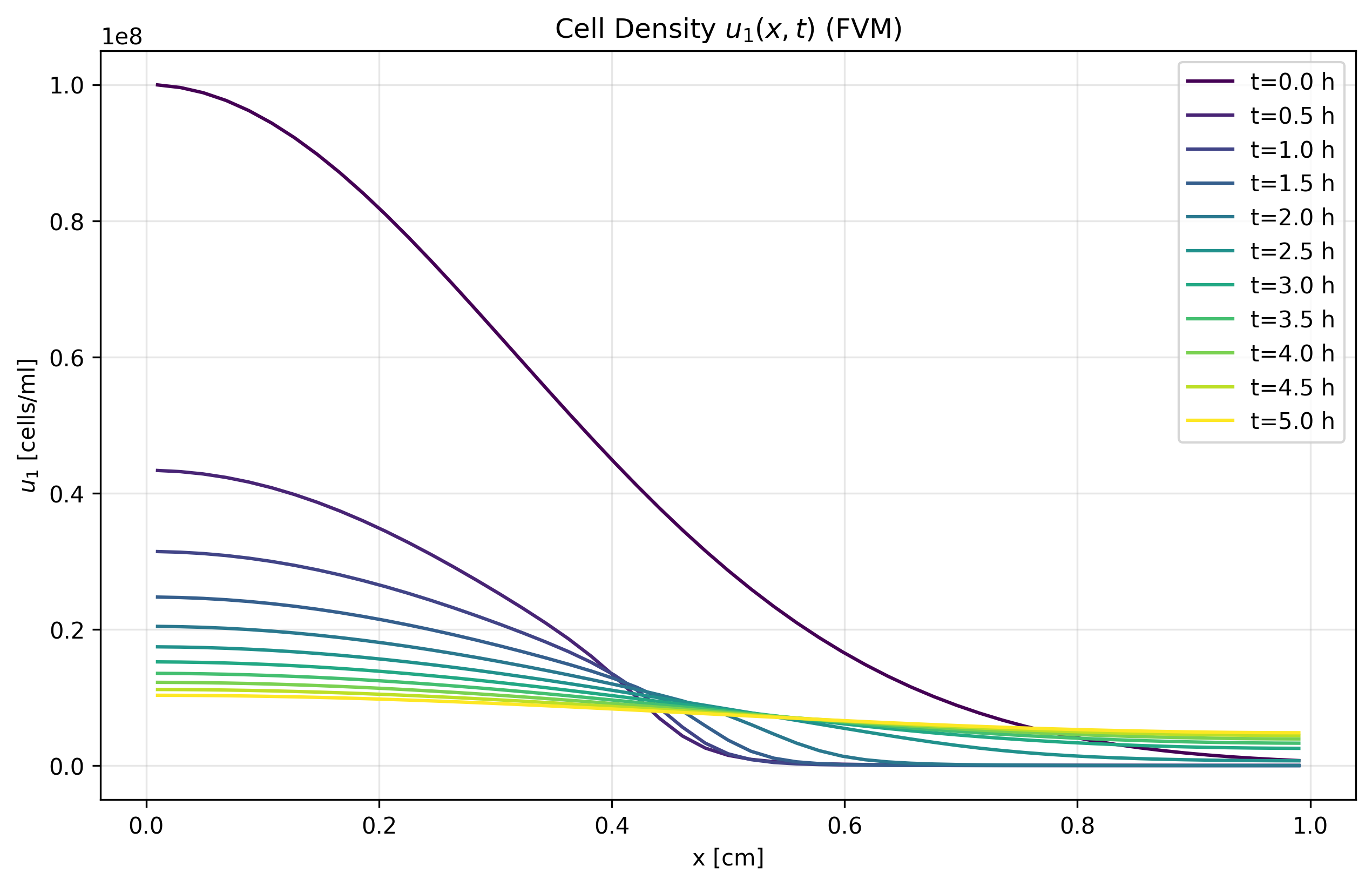
Figure 1a: u₁ FVM Solution
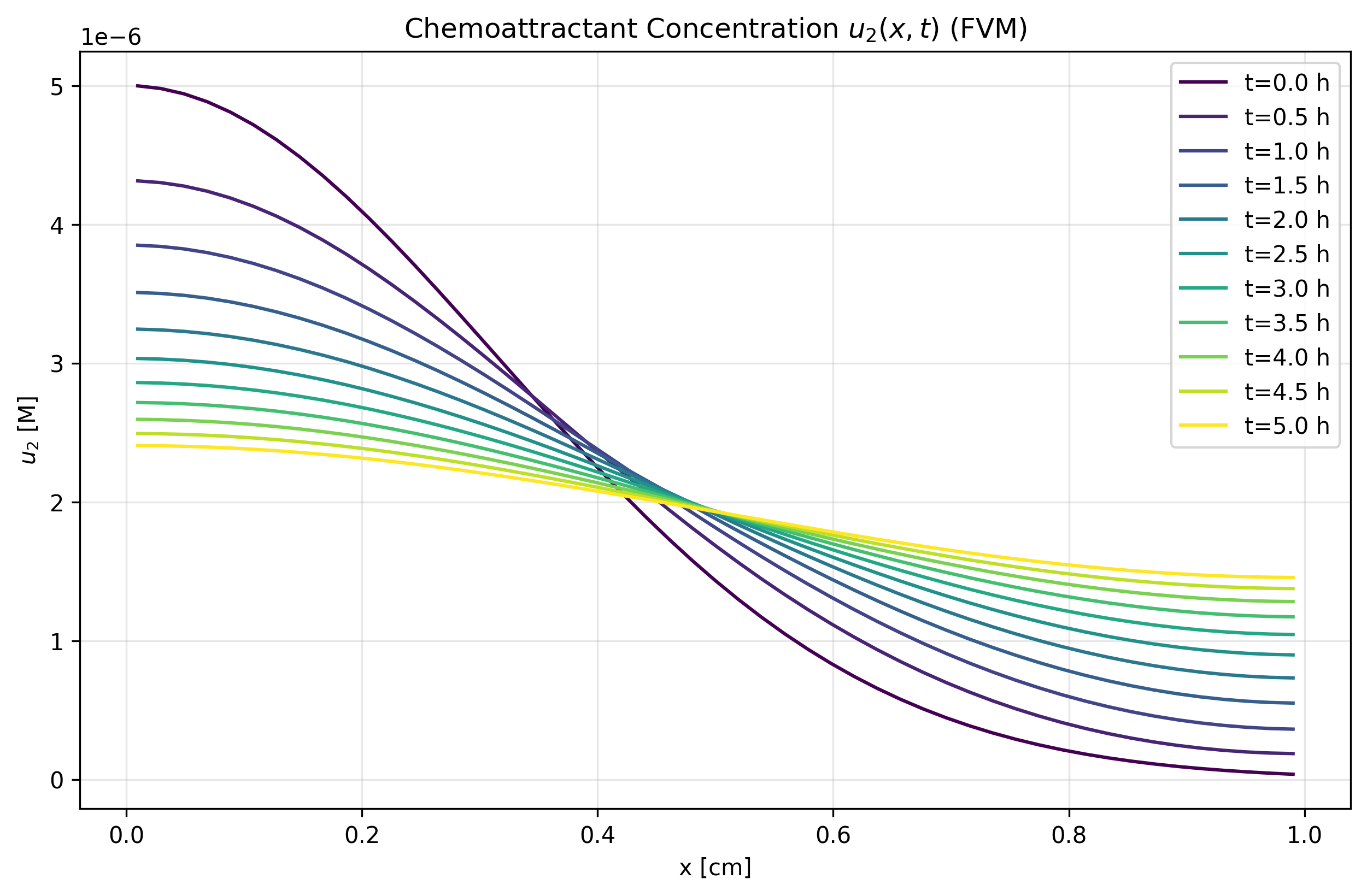
Figure 1b: u₂ FVM Solution
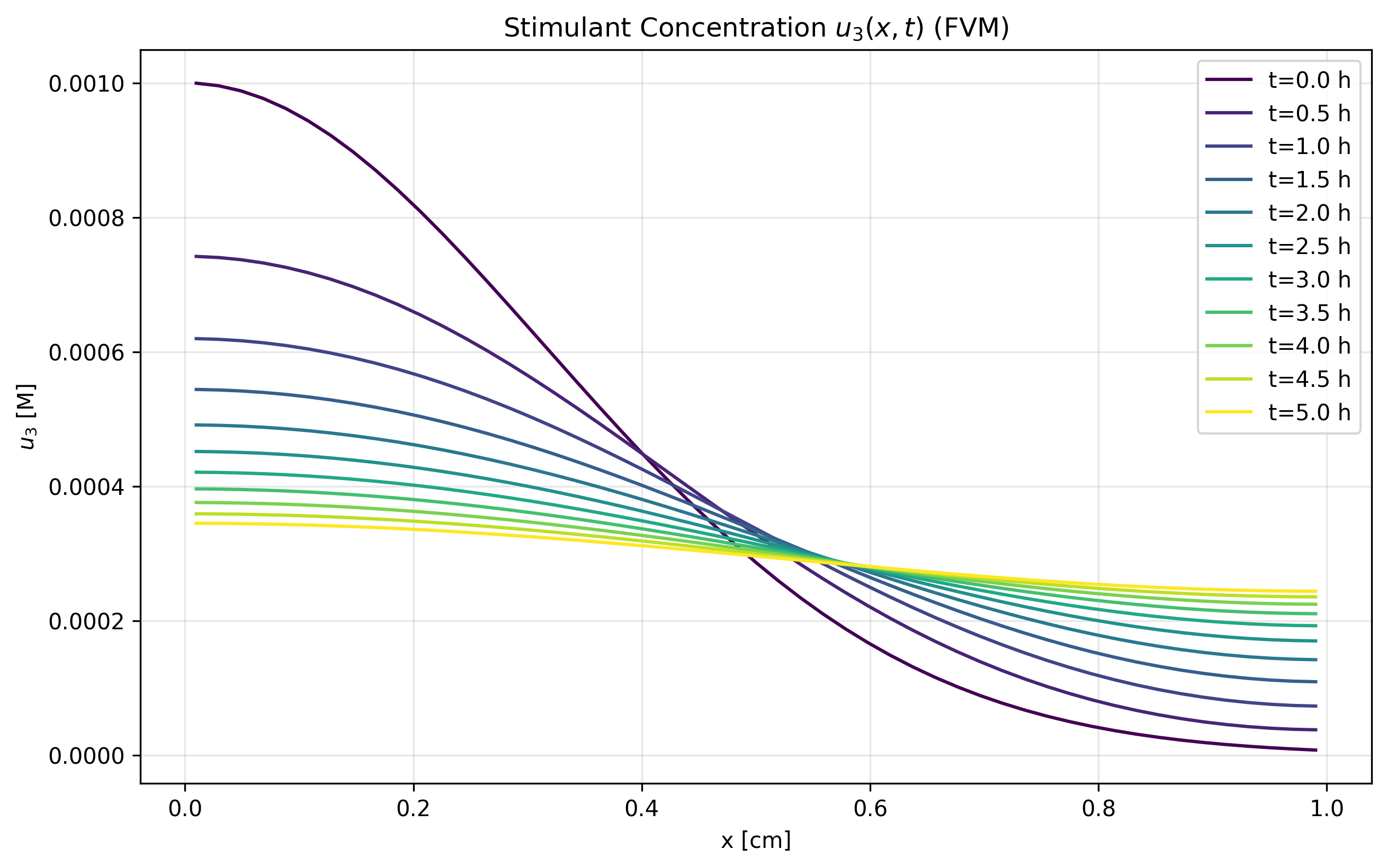
Figure 1c: u₃ FVM Solution
Machine Learning Approach
Implementation Steps
Our ML-enhanced PDE solver implements the following workflow:
PDE Model Conversion
- Implemented biological equations through PatternFormationPDE class
- Defined parameters: diffusivities (D₁, D₂, D₃) and rate constants (k₁-k₉)
Spatial Discretization
- Created 1D grid with 51 support points (\(x \in [0,1]\) cm)
- Applied Neumann boundary conditions (zero-flux)
- Initialized with Gaussian state: \(u_1(x,0) = 10^8e^{-5x^2} \) cells/mL
Adaptive Time-Stepping
- Used Scipy's BDF solver for stiff systems
- Stored solution states at 0.5hr intervals
- Calculated diffusion, chemotaxis, and stimulation terms
Solution Analysis
- Extracted and visualized spatiotemporal patterns
- Printed final state at t = 5 hours
- Compared accuracy against reference solutions
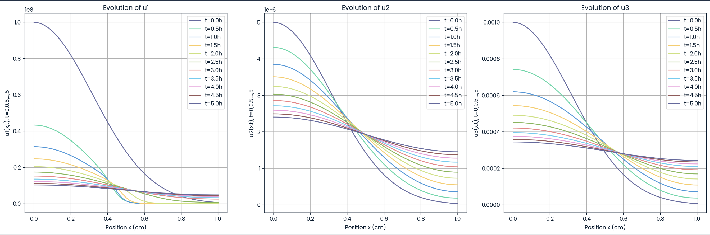
Results at t = 5 hours
| x (cm) | u₁ (cells/mL) | u₂ (M) | u₃ (M) |
|---|---|---|---|
| 0.0 | 1.0296 × 10⁷ | 2.4961 × 10⁻⁶ | 3.4552 × 10⁻⁴ |
| 0.2 | 9.7859 × 10⁶ | 2.3936 × 10⁻⁶ | 3.3582 × 10⁻⁴ |
| 0.4 | 8.3396 × 10⁶ | 2.1425 × 10⁻⁶ | 3.1154 × 10⁻⁴ |
| 0.6 | 6.6273 × 10⁶ | 1.8362 × 10⁻⁶ | 2.8066 × 10⁻⁴ |
| 1.0 | 4.9208 × 10⁶ | 1.4863 × 10⁻⁶ | 2.4373 × 10⁻⁴ |
Evolutions of u₁, u₂, and u₃

Figure: Spatiotemporal evolution of pattern formation
Relative Errors at Selected Points
| x (cm) | u₁ (cells/mL) | u₂ (M) | u₃ (M) |
|---|---|---|---|
| 0.0 | 0.43 | 0.65 | 0.18 |
| 0.4 | 0.08 | 0.45 | 0.02 |
| 0.8 | 0.46 | 0.72 | 0.18 |
Key Findings
- The ML approach achieves high accuracy (≤1.98% error) while efficiently solving 153 coupled ODEs
- Pattern formation dynamics are accurately captured across all three fields (cell density, chemoattractant, stimulant)
- Solution snapshots stored every 30 minutes enable detailed temporal analysis
- The method demonstrates robustness in handling complex biological interactions
- Good agreement with traditional numerical methods validates the approach
- Significant potential for scaling to higher-dimensional problems
Summary Disscusion
Solution Accuracy Comparison
This section compares the accuracy of our three solution approaches against reference results from literature. Each table shows the maximum and minimum percentage errors for the three system variables (u₁: Cell Density, u₂: Chemoattractant, u₃: Stimulant) relative to established benchmark solutions.
Learning-Based Method
| Field | MAX Error (%) | MIN Error (%) |
|---|---|---|
| u₁ | 1.98 | 0.04 |
| u₂ | 0.72 | 0.36 |
| u₃ | 0.18 | 0.01 |
Finite Volume Method
| Field | MAX Error (%) | MIN Error (%) |
|---|---|---|
| u₁ | 0.59 | 0.07 |
| u₂ | 3.11 | 1.61 |
| u₃ | 0.17 | 0.02 |
Finite Difference Method
| Field | MAX Error (%) | MIN Error (%) |
|---|---|---|
| u₁ | 0.17 | 0.03 |
| u₂ | 2.98 | 1.75 |
| u₃ | 0.03 | 0.01 |
Computational Performance
The table below compares the computational efficiency of the different solution approaches. Runtime is measured in seconds for the full simulation, with problem size quantified by the number of ordinary differential equations (ODEs) solved.
| Metric | MOL | LEARNING-BASED | FVM | FDM |
|---|---|---|---|---|
| Runtime (sec) | 1.826 | 6.446 | 1.132 | 1.881 |
| Problem Size (no. of ODEs) | 153 | 153 | 153 | 153 |
| Time per Equation (s/equ) | 0.0119 | 0.0452 | 0.0074 | 0.0123 |
| Function Evaluations | 1052 | 3717 | 945 | 1052 |
Future Work and Improvements
Algorithmic Enhancements
Adaptive Mesh Refinement
Implement h-refinement to dynamically increase spatial resolution in regions of steep gradients
High-Order Integration
Upgrade to 6th-order finite difference schemes to reduce discretization errors
Model Extensions
2D/3D Simulations
Extend to higher dimensions to model realistic biological pattern formation
Stochastic Terms
Introduce noise to model microenvironment variability and heterogeneity
Neural ODEs
Implement data-driven parameter calibration using neural ODE frameworks
Deep Learning Integration
Hybrid Solver
Incorporate microscopy data via CNN encoders to generate biologically realistic initial conditions
Operator Learning
Train Fourier Neural Operators to predict patterns without solving full PDEs
Uncertainty Quantification
Implement Bayesian PINNs to estimate solution confidence intervals
Biological Applications
Cancer Research
Model tumor invasion patterns and metastasis formation
Drug Delivery
Simulate smart drug navigation through biological systems for targeted therapies
Acknowledgment
The authors would like to express their sincere gratitude to their course supervisor, Professor Muhammad Rushdi, for his invaluable guidance, encouragement, and support throughout this project, which was conducted as part of the Numerical Methods course at Cairo University.